Tuesday, December 30, 2014

Integrating an Android smartphone application with the BLED112 module

My conclusion with the RFDuino adventures was that RFDuino is a perfect platform to start familiarizing with the Bluetooth Low Energy (BLE) technology. BLE programming was made so simple with RFDuino that it provides quick success. Simplification comes with limitations, however, and eventually time has come for me to step further toward a more flexible BLE platform. Bluegiga's BLE121LR long range module seems to have outstanding range but first I tried a piece of hardware that is equivalent from the API point of view with the BLE121LR but is easier to start with and that is Bluegiga's BLED112 USB dongle.


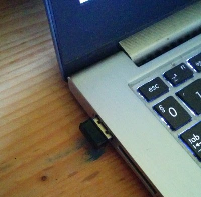
The BLED112 implements the same API (called BGAPI, check out Bluetooth Smart Software API reference) that other Bluegiga BLE modules do but there's no need to buy the pricey DKBLE development board or build any hardware. It plugs neatly into the USB port and is functional without any additional piece of hardware. From the serious BLE application development perspective it has drawbacks too. Firstly, its USB interface is drawing a constant 5mA current so this solution is not very much "low energy". Second disadvantage is that its single USB interface is shared between the BGAPI API and the programming interface so installing scripts into the BLED112 is a risky enterprise. If the script running on the BLED112 occupies the USB port, there's no way to update it so the module is essentially bricked. Hence in this exercise we will keep the BLE application logic on the PC hosting the module and talk to the module with BGAPI. This is very similar setup when the application logic is running on a microcontroller or embedded PC.

Click here to download the Android client and the PC server example programs.

In this exercise, we will implement the Current Time Service (CTS) and access this service from an Android application. CTS is a standard Bluetooth service. The PC application will fetch the current time from its clock and will update the characteristic exposed by the BLED112. The Android application will detect the advertised CTS service, connect to it, retrieve the time and display it to the user. The Android application will also subscribe to time changes demonstrating the notification feature of BLE GATT.

Let's start with the PC part. Unpack the cts_example.zip file and inside there are a set of C files belonging to the PC application in the root directory. I developed and tested the application on Ubuntu 14.10 so if you use a similar system, you have good chances that you just type "make" and it will compile. Preparing the BLED112 dongle is more complicated, however and this is the result of the quite cumbersome Bluegiga tool chain. Any change to the GATT services (read this presentation if you don't know what GATT is) requires a firmware update of the BLED112. This sounds scary but it is not too complicated if you have a Windows system. Bluegiga SDK supports only Windows and there is one element of the tool chain, the firmware downloader that does not run on emulated Windows either - you need the real thing. So the steps are the following:

  • Grab a Windows machine, download the Bluegiga SDK and install it.
  • Get the content of the config subdirectory in cts_example.zip and copy somewhere in the Windows directory system. Then generate the new firmware with the <bluegigasdk_install_location>\bin\bgbuild.exe cts_gattBLED112_project.bgproj command. The output will be the cts_BLED112.hex file which is the new firmware. We could have placed application logic into the firmware with a script but as I said, it is a bit risky with the BLED112 so this time the new firmware contains only the GATT database for the CTS service.
  • Launch the BLE GUI application, select the BLED112 port and try to connect by clicking the "Attach" button. If all goes well, you will see green "Connected" message. Then select Commands/DFU menu item, select the HEX file we have just generated, click on the "Boot into DFU mode" button. One pecularity of the BLED112 that in DFU mode it becomes logically another USB device so the main window will display red "Disconnected" message.  Then click "Upload". If the upload counter reaches 100% and you see the "Finished" message, the firmware update is done.
At this point we are finished with Windows and can start the serious business. Plug the dongle into the Ubuntu machine and check out its port.

dmesg | tail
...
usb 3-2: Product: Low Energy Dongle
usb 3-2: Manufacturer: Bluegiga
usb 3-2: SerialNumber: 1
cdc_acm 3-2:1.0: ttyACM0: USB ACM device


So this time the dongle is mapped to /dev/ttyACM0. Launch the BLE server with the following command:


./conn_example /dev/ttyACM0


The server is ready, let's see the Android client. Import the Android project in CTS.zip into Android Studio. Note that I am still baffled by the fact that this shiny new IDE does not have a project export command so I had to zip part of the project's directory tree manually. Once you launch the Android application, you will see a screen like this:


The device named "test" is our device and the CTS service is identified by the UUID of 0x1805. The other entry is just another BLE device that I threw in for demonstration. Click on the device name and you get the time emitted by the BLE dongle:


The current time is also updated every second demonstrating that the client successfully subscribed to the changes.


On the server side, it is important to note that the BGAPI protocol is defined in terms of byte arrays sent and received over the serial port (which is mapped to USB in the case of BLED112). The BGAPI support library coming from Bluegiga that I used in this demo is just a wrapper over this interface so it can be replaced with an optimized implementation if the library is too heavy for the application platform (e.g. for a microcontroller) or is not implemented in the desired language (e.g. in Python). On the Android client side, it is interesting to note how the BLE advertisement parser library I presented in this post is used to figure out, whether the device advertises the CTS service we are interested in.

Friday, December 19, 2014

Parsing BLE advertisement packets

Ever since I created the Gas Sensor demo (post here, video here, presentation here), I had the feeling of an unfinished business. That demo sent the sensor data in BLE advertisement packets so the client never connected to the sensor but received data from the sensor in a broadcast-like fashion. The implementation looked like this:

        public void onLeScan(final BluetoothDevice device, int rssi, byte[] scanRecord) {
            String deviceName = device.getName();
...
                int addDataOffs = deviceName.length() + 16;
                int siteid = ((int)scanRecord[addDataOffs]) & 0xFF;
                int ad1 = ((int)scanRecord[addDataOffs+1]) & 0xFF;

This was a quick & dirty solution that remained there from my earliest prototypes. It sort of assumes that the structure of the BLE advertisement packet is fixed so the sensor data can always be found at fixed locations of the advertisement packet. This does not have to be the case, Bluetooth 4.0 Core Specification, Part C, Appendix C (or Core Specification Supplement in case of 4.2 version) describes, how the fields of the advertisement packets look like. It just so happens that with the given version of the RFDuino BLE module, the Manufacturer Specific Data field where RFDuino puts the user data for the advertisement packet can always be found at a specific location.

The proper way is of course to parse this data format according to the referred appendix of the specification and in this post I will show you how I implemented it.

Here are the three example programs mentioned in this post: blescan.zip, gassensordemo.zip, gas_adv.ino

Let's see first the BLEScan project.

Update: the project has been updated to support more of the 4.2 elements. It has also been converted into an Android Studio project but the download material contains only the app/src part of the tree.

Update: I was asked by e-mail, how to import the project (in blescan.zip) into Android Studio. Here is a simple process.
  • Create a new project in Android Studio under any name. Make sure that your project supports at least API level 18. Choose the "create no Activity" option.
  • Once your project is created, go and find it on the disk. On my Ubuntu system, the project files go under ~/StudioProjects/<ProjectName> where <ProjectName> is the name you gave to your project. We will call this directory <ProjectDir>.
  • Go into <ProjectDir>/app/src and delete everything there. Copy blescan.zip into <ProjectDir>/app/src and unzip it. It will create a single directory called "main" and the sources below.
  • In Android Studio, do File/Synchronize. After that is completed, you can open your project files, build APK, etc.

The parser code is under the hu.uw.pallergabor.ble.adparser package. Then you just give the scanRecord array to AdParser's parseAdData method like this:

            ArrayList<AdElement> ads = AdParser.parseAdData(scanRecord);

and then you get an array of objects, each describing an element in the scan record. These objects can also produce printable representation like this:


Now let's see the revised GasSensorDemo project, how the gas sensor measurement is properly parsed out of the scan record. First we parse the scan packet fields:

                ArrayList<AdElement> ads = AdParser.parseAdData(scanRecord);

Then we look for a TypeManufacturerData element which corresponds to a Manufacturer Specific Data field in BLE. We make an extra check to make sure that the manufacturer field in the Manufacturer Specific Data is 0x0000 because RFDuino always creates a Manufacturer Specific Data field like that if the application programmer specifies additional advertisement data.

                    AdElement e = ads.get(i);
                    if( e instanceof TypeManufacturerData ) {
                        TypeManufacturerData em = (TypeManufacturerData)e;
                        if( em.getManufacturer() == 0x0000) {


It would be tempting to use a custom manufacturer field or better, a Service Data field. But then we run into another limitation of RFDuino because RFDuino with its default firmware is only able to create advertisement packets like in the previous example. This is not bad because it allows the programmer to achieve quick success but later on, we will need more flexibility and that will need another BLE module.

Friday, November 21, 2014

Motor boat control with Bluetooth Low Energy

 My previous post about Bluetooth Low Energy applications with RFDuino and Android presented a connectionless gas sensor. That prototype was based solely on BLE advertisements, no connection was built between the scanner device (Android phone or tablet) and the sensor. While this connection-less operation is advantageous for sensors that just broadcast their measurement data, more complex scenarios that e.g. require authentication or build a communication session cannot be implemented in this model. The prototype I am going to present in this post demonstrates connection-oriented operation between RFDuino and an Android application.

Watch this video to see what the application is about.


The story behind this motor boat project is that I bought this RC-controlled model boat while I worked in the UK. But when we moved back to Hungary, I lost the RC controller. So the boat had been unused for years until I realized how great it would be to use an Android device as a controller. Hence I quickly integrated the RFDuino with the motor boat's original control circuitry and wrote the necessary software. As you can see in the video, it has quite respectable range even though I did not dare go into the October water of Lake Balaton where the second part of the video was shot (water temperature: some 10 degrees centigrade).

First about the "hardware". I did not have the circuit schema of the original RC controller in the boat so I had to experiment a bit. By following the motors' cables I quickly found two three-legged stocky elements that looked like switching transistors (although the labels on them were not readable after all those years in service). I removed one end of the resistors that I thought connected the base of these transistors to the rest of the RC control circuit and tried out, how much current is needed to switch on the motors. To my pleasant surprise, 1 mA current was enough so I rather believe that these are actually not transistors but power switching ICs. Anyway, RFDuino outputs can provide 1 mA switching current so I just connected the other end of those removed resistors to two spare RFDuino I/O ports. Lo and behold, it worked. If RFDuino raises any of these pin to 1, the respective motor starts. One minor additional problem was about the power supply of RFDuino. The motor boat employs an 7.2 Volt battery and RFDuino needs 3.3 V. I added an LM1117-3.3V power regulator circuit between the battery and RFDuino and the "hardware" was ready.


Do you know about BLE concepts like service and characteristics? If not, please read this presentation for a quick introduction. In short: BLE services (also called GATT profiles) are composed of characteristics which are key-value pairs decorated by meta-information that the BLE specification calls descriptors. RFDuino with its default firmware is not able to implement any standard GATT profile except for its own custom GATT profile. This is a major disadvantage in product-level development but makes RFDuino code super-easy because the programmer does not have to deal with BLE details. In the RFDuino custom service, a "read" and a "write" characteristic is defined. Whatever the client (in our case, the Android application) writes into the "write" characteristic appears for the RFDuino code as incoming data callback. If the RFDuino code calls the RFduinoBLE.send(v) method, the data appears in the "read" characteristic. The Android client can register a callback for data manipulations of the "read" characteristic so it will receive callbacks when RFDuino code invokes the RFduinoBLE.send() method. There are additional callbacks for service connections and disconnections.

You can download the Android project and the RFDuino source here.

First about the RFDuino code.  Beside the familiar setup() and loop() functions, you will see three functions characteristic to RFDuino. RFduinoBLE_onConnect() is called if a client connects to the RFDuino BLE service, RFduinoBLE_onDisconnect() is called on disconnection and RFduinoBLE_onReceive() is called when there is incoming data. There is only one complication in the code that requires explanation: this is a powerful motorboat and it can go out of BLE radio range very quickly. In the early versions the boat became uncontrollable in this case meaning that it just continued with the last command received. That was not a nice feature so I implemented a heartbeat message feature which is sent in every 5 second. The loop() method starts by sending the heartbeat to the client and goes to sleep. It wakes up after 5 seconds and if it finds that the client did not send back the heartbeat, it stops the motors. Otherwise the client just sends a bit mask about which motors to stop or start and the RFDuino just responds with the same mask informing the client that the motors were indeed started or stopped. This means that the arrows on the user interface showing which motors are running represent the actual state of the boat which is advantageous if something goes wrong.

Then about the Android side. The code starts by discovering the device. Once the device is discovered, we connect to the device with the connectGatt() method then discover its services with gatt.discoverServices() method. Once the service discovery callback arrives, we retrieve the RFDuino service (getService(), we expect this custom service) and obtain the characteristic handles (getCharacteristic()). We use the "read" characteristic's client configuration descriptor to enable notifications from the RFDuino server to the Android client so that we get a callback when the RFDuino side sends something to us.

Disconnection is worth detailing because there's an RFDuino speciality here. Normally, one can just disconnect from the service with the disconnect() method invocation. RFDuino however is left in a limbo state in this case: the BLE session is disconnected but the RFDuino application does not receive a callback and cannot accept a new connection request. The "disconnect" characteristic has to be written to (the value does not matter) for the RFDuino server to properly disconnect.

Friday, October 3, 2014

Award for our Android Gas Sensor

I just got a mail that our gas sensor entry (a gas sensor with Bluetooth Low Energy connectivity and the associated Android application) has just won 3rd place on the We Know RFDuino contest. Thanks to everyone who viewed our video and thus helped us to compete successfully! Meanwhile the source code of the prototype was made open source so you may want to check out that too!

Monday, September 29, 2014

Gas sensor prototype explained

The "We know RFDuino" contest has not ended yet but its end is sufficiently close so that I can explain our prototype application. Our entry is a Bluetooth Low Energy-connected gas sensor and it is presented in the video below. Make sure that you watch it, you help us win the competition.


The prototype demonstrates a unique capability of Bluetooth Low Energy device advertisement messages: you can embed user data into these broadcasts. These come handy if you just want to send out some measurement data to whoever cares to listen without creating a session between the BLE client and server. This broadcast-type data transfer may support unlimited number of clients with very low energy consumption on the sensor side.

Click here to download the Android client application project.

Click here to download the RFDuino source code.

The prototype works like the following. The microcontroller presented in the video measures the Lower Explosion Limit and sends this value to the RFDuino microcontroller over a super-simpe serial protocol. A message of this protocol looks like this:

0xA5 <seq_no> <LEL%>

where seq_no is an increasing value and LEL% is the measured Lower Explosion Limit value. The microcontroller code is not shared here but you can get the idea. The RFDuino code receives the LEL% value over the serial port it creates on GPIO pins 3 and 4, creates a custom data structure for BLE advertisements consisting of the site ID and the LEL% value then starts advertising. This is performed cyclically so the LEL% value is updated in the sensor's BLE advertisement every second.

Now let's see what happens on the Android side. This is a non-trivial application with multiple activities but the Real Thing (TM) happens in the MapScreenActivity, in the onLeScan method. This method is called every time the Android device's BLE stack discovers a device. In this case we check whether the device's name is "g" (this is how we identify our sensor) and we retrieve the LEL% data from the advertisement packet.  We also handle the Received Signal Strenght Indicator (rssi) value for proximity indication. Bluetooth device discovery is restarted in every 2 seconds so that we can retrieve the latest LEL% value. The rest is just Plain Old Android Programming.

The identification of the sensor and the encoding of the sensor data is obviously very naive but this is not really the point. You can make it as complex as you like, e.g. you can protect the sensor data with a hash and place that hash also into the advertisement so that the receiver can make sure that it gets data from an authorized sensor and not a fake one. The important thing is that the entire framework is sufficiently flexible so that relatively complex functionality can be implemented and RFDuino really simplifies sensor programming a lot.

If you enjoyed the example application, make sure you watch the video (many times if possible :-)) and if you happen to be in London on 2014 November 19, you might as well come to the Londroid meetup where I present this and another BLE project (a connection-oriented one, called MotorBoat).

Saturday, September 6, 2014

Camera shot on charger connection

Somebody came to me with an idea whether a cheap Android phone can be turned into an automatic camera. Some external sensor would send a signal to the phone and the phone would take a picture automatically. We started to discuss the possible connection of the external sensor and an interesting idea came up: the charger connection.

Android delivers an event whenever the charging power is connected or disconnected: can it be used to send a binary signal to an application in a very simple way, without fiddling with Bluetooth or USB?

Click here to download the example application.

You have to start the application once. Then whenever you connect the charger, it takes a picture. When the application is in the foreground, a preview is shown but as long as the application is active (not destroyed) it works from the background too.

Here are the experiences:

  • On my high-end device the application reacted quickly to charger connection, the reaction time from connecting the charger to the camera shot was less than a second. But when the application was tested on the very low-end Android target device, the picture was much less rosy: the delay increased to 3-4 seconds, effectively making the solution unusable.
  • In order for this application to work, it has to be started at least once manually. This pretty much kills all unattended use cases.
  • The shutter sound is almost impossible to remove. Update: on certain devices (Nexus 4 and Nexus 7 confirmed) there is no shutter sound in silent mode.
The takeaway for us was to reject the idea. But I share the example program anyway, maybe it can be useful for somebody.


Tuesday, September 2, 2014

Android gas sensor application with Bluetooth Low Energy/RFDuino

I have always had a fascination with sensors linked up with mobile devices so it seemed just a good opportunity to try out the latest fashionable technology in the area, Bluetooth Low Energy in the context of a competition. SemiconductorStore.com announced the "We know RFDuino" competition for applications of the RFDuino module. RFDuino is an Arduino module with Bluetooth Low Energy (BLE) support. It is ideal to act as an interface between a sensor and a BLE-enabled mobile device like the Nexus 7.

Eventually I will publish the entire source code of this prototype application on this blog. But as this is a contest, I will wait until the contest ends (Sept. 30). Till then, watch the (very amateurish) video we have prepared about our sensor and the Android application. The entry with the most views wins the contest so if you like the concept, share the video with others! Thanks in advance. :-)


Tuesday, March 11, 2014

Beyond RenderScript - parallelism with NEON


My last post about the parallel implementation of Distributed Time Warping (DTW) algorithm was a disappointment. The RenderScript runtime executed the parallel implementation significantly slower than the single-core implementation (also implemented with RenderScript). It turned out that parallelizing the processing of 10000-50000 element vectors on multiple cores were not worth the cost of the multi-thread processing and all the overhead that comes with it (threads, semaphores, etc.). One core must be allocated a significantly larger workload but our DTW algorithm is not able to generate such a large, independent workload because rows of the DTW matrix depend on each other. So in order to exploit RenderScript multi-core support, it is best to have an algorithm where the output depends on only the input and not on some intermediate result because this type of algorithm can be sliced up easily to multiple cores.

It would have been such a waste to discard our quite complicated parallel processing DTW algorithm so I turned to other means of parallel execution. Multi-core is one option but the ARM processors in popular Android devices have another parallel execution engine, internal to the core, the NEON execution engine. One NEON instruction is able to process 4 32-bit integers in parallel (see picture below). Can we speed up DTW fourfold with this option?


NEON is actually quite an old technology, even Nexus One was equipped with it. It is much more widely deployed therefore than multi-core CPUs. While ordinary applications can take advantage of multi-core CPUs (e.g. two processes can execute in parallel on two cores), NEON programs are difficult to write. Although some compilers claim the ability to generate NEON code and template libraries are available, the experience is that the potential performance benefits cannot be exploited without hand-coding in assembly and that's not for the faint hearted.

The example program can be downloaded from here.

The relevant functions are in jni/cpucore.c. There are 3 implementations, processNativeSlow, processNative and processNativeNEON, each is progressively more optimized than the previous one. The processNativeSlow and processNative functions are in C, in processNativeNEON the most time-critical loop ("tight loop") is entirely implemented in mixed ARM/NEON assembly. This tight loop produces 4 result elements in parallel so we expect huge performance gain over the single-core RenderScript implementation (dtw.rs).

The experience is completely different. While the NEON implementation is significantly faster on small datasets, one second of voice is 8000 samples so data sizes grow quickly. On 10 second data sets (80000 samples, 6.4 billion element DTW matrix) the simple nested loop C99 implementation and the complex, hard to understand NEON implementation produces about the same execution time.

How is this possible? Let's take an example of 10 second reference and evaluation samples. This means 80000 elements, 80000*80000=6.4 billion values to calculate. Calculating each value takes 20 bytes to access (2 input samples (2 bytes each), 3 neighbor cells (4 bytes each) and storing the result (4 bytes)). A1 SD Bench measures 800 Mbyte/sec copying performance on my Galaxy Nexus (and similar values on the two cheap Android tablets that the family has), that obviously means 2 accesses (one read and one write). For simplicity, let's assume that reads and writes take about the same time. This means that according to this very rough calculation, the memory accesses themselves take about 80 sec. The real execution time is about 120 sec, the difference can be explained by the simplifications. Cache does not really help because of the large data size. The performance is determined by the RAM speed and the simplest single-core implementation already reaches the bottleneck. All the wizardry with parallelism is futile.

Obviously the case was not helped by the selection of the DTW algorithm as benchmark which intentionally does not fit into the class of algorithms normally used to demonstrate the benefits of parallel processing. Grayscale conversion would be better (one read, one write and 3 multiplications per pixel). But this means that you actually have to be really lucky with your algorithms for these parallel options to speed up your code significantly. Even then, it is worth looking at the parallel options inside the core before going multi-core. And you definitely should not forget the auxiliary costs of parallel computation, e.g. distributing/gathering the data to/from the parallel processing units or whether other hardware (e.g. memory) is able to keep the pace with the CPU.

One wild idea at the end. Could RenderScript computation model be used to generate NEON code? With some limitations, the answer is probably yes.

Friday, February 7, 2014

RenderScript in Android - the parallel version

In the previous post I promised to revisit the parallel case. The big promise of RenderScript is to exploit parallelism among different CPUs, GPUs and DSPs in the device at no additional cost. Once the algorithm is properly transformed into parallel version, the RenderScript runtime grabs whatever computing devices are available and schedules the subtask automatically.

The problem with DTW is that it is not so trivial to parallelize. Each cell in the matrix depends on cells at (x-1,y), (x-1,y-1) and (x,y-1) (provided that the cell to calculate is at (x,y)). By traversing the matrix horizontally or vertically, only two rows (one horizontal and one vertical) can be evaluated in parallel.

Michael Leahy recommended a paper that solves this problem. This algorithm traverses the matrix diagonally. Each diagonal row depends on the two previous diagonal rows but cells in one diagonal row don't depend on each other. One diagonal row can be then fed to RenderScript to iterate over it. The picture below illustrates the concept.


The example program can be downloaded from here.

You will notice that there are two parallel implementations. The findReferenceSignalC99Parallel() is the "proper" implementation that follows closely the RenderScript tutorial. Here the diagonal rows are iterated in Java and only the parallel kernel is implemented in RenderScript. This version - even though it is functional - is not invoked by default because it delivers completely inacceptable performance on my 2-core Galaxy Nexus. By looking closely at the execution times, I concluded that even though RenderScript runtime invocations ( copying into Allocations and invoking forEach) are normally fast, sometimes very innocent-looking invocations (like copying 5 integers into an Allocation) can take about a second. This completely ruined this implementation's performance.

The other parallel implementation which is actually invoked and whose performance is compared to the 1-core RenderScript implementation (the fastest one) is findReferenceSignalC99ParallelRSOnly(). This version is implemented entirely in RenderScript. Unfortunately its performance is 2-2.5 times slower than the 1-core implementation. How can it be?

First, if you compare dtw.rs and dtwparallel2.rs, you will notice that the parallel implementation is considerably more complex. Indexing out those varying-length diagonal rows takes a bit of fiddling while the 1-core implementation can take the advantage of fast pointer arithmetic to move from cell to cell sequentially. So the parallel implementation starts with a handicap. This handicap is not compensated by the 2 cores of the Galaxy Nexus.

OK, Galaxy Nexus is the stone age but what happens on a 4-core processor like on a Nexus 4? The runtime does launch with 4 cores but then the Adreno driver kicks in and the result is that the parallel implementation is about 3 times slower than the serial one. What happens in the driver, I don't know, as far as I can see, the source code is not available.

Jasons Sams recommended to disable the GPU driver with
adb shell setprop debug.rs.default-CPU-driver 1
but I decided to stop my adventures here. The conclusion I drew for myself is that RenderScript in its present form is not ready for parallel programming. Clang-LLVM is a very promising compilation technology but the parallel runtime suffers from a number of problems. IMHO, there should be a way to programmatically control the way the workloads are allocated to CPUs/GPUs. Until then, if you want to harness the power of your multicore processor, code the parallel runtime yourself. Using RenderScript for the serial code if you wish.

Thursday, January 30, 2014

RenderScript in Android - anatomy of the benchmark program

 In the previous post I have presented our RenderScript benchmark and demonstrated that RenderScript implementation of the same algorithm can be 2-3 times faster than Java. How can a "script" be so fast? In order to understand this speed difference, let's see how the RenderScript fragment is executed.

The example program is available here.

First, let's see how the script looks like. The source can be found in dtw.rs, in the same directory where other Java sources (just one file in this case) are.


It looks like an innocent C function but there are some specialties. All the global variables like these ones:

int32_t s2len = 0;
int32_t *d0;


can be used to pass data to the script.  The toolchain generates a Java wrapper for each .rs file, ours is called ScriptC_dtw.java. In order to set s2len, for example, one calls the set_s2len function in the ScriptC_dtw class. The d0 global variable is a pointer type, setting this variable requires an Allocation Java object. Open MainActivity.java and look up the findReferenceSignalC99() method. There you will find:

        Allocation signal1Allocation = Allocation.createSized(
                rsC,
                Element.I16(rsC),
                refSignal.length);
        signal1Allocation.copyFrom(refSignal);
        script.bind_signal1(signal1Allocation);


Here we created an allocation that holds 16-bit integers, copied the input signal into it and bound the allocation so that the allocation's data is available to the script. When the script is invoked, the data area of this allocation is simply available to the script as:

int16_t *signal1;

This sort of parameter passing is one-way for simple values but two-way for allocations. So whatever you write in your script into e.g. s2len, you won't be able to read it in the Java layer after the script finishes executing. In contrast, Allocations provide two-way data transfer, that's why the result value is passed back to Java in an Allocation.

In MainActivity.java:

        Allocation rAllocation = Allocation.createSized(
                rsC,
                Element.I32(rsC),
                1);
        script.bind_r(rAllocation);


In dtw.rs:

        *r = d1[s1len-1];

And again in MainActivity.java after the script finished executing:

        int result[] = new int[1];
        rAllocation.copyTo(result);
...
        int maxc = result[0];


The execution of the script seems simple enough but there's more than meets the eye.

Execution context and the script instance are created.

        RenderScript rsC = RenderScript.create( this);
        ScriptC_dtw script = new ScriptC_dtw(
                rsC,
                getResources(),
                R.raw.dtw);


ScriptC_dtw is the wrapper which was generated by RenderScript toolchain. But what is R.raw.dtw? Let's see how our "script" was turned into executable code. If you unzip the APK file, you find some interesting artifacts. Under the res/raw directory, you find dtw.bc. This is the LLVM bytecode that dtw.rs was compiled to. In addition, under the lib directory, you will find .so files for the ARM, MIPS and Intel platform. If you disassemble librs.dtw.so, you will find highly optimized binary compiled from our script which is really a piece of valid C code.


The RenderScript name generates a confusion. This name evokes a proprietary scripting language when in fact it is Clang's C99 front-end compiler with a set of libraries that are ported to a large number of processors. Optimized C code is fast, what is so surprising in it? When our "script" is executed on an ARM processor, the RenderScript runtime just has to load the precompiled ARM code and execute it. If it turns out that there is no precompiled native code for the target processor (e.g. it is a GPU) then LLVM backend compiler swings into action and generates code for that processor at installation time. Both compilation steps (from C to LLVM bytecode and from LLVM bytecode to native) are subject to optimization so the resulting native code is very fast. No wonder therefore that RenderScript beats Dalvik VM so easily and with such a large margin.

After all the global variables have been initialized, the script can be invoked.

        script.invoke_dtw();
        rsC.finish();


Note the finish() invocation here. The invoke_dtw() method is asynchronous meaning that when it returns, the execution of the "script" has not finished, in fact, it was not even started. The finish() method on the RenderScript instance blocks until the script invocations on that context all finish. Script invocations in the same context are executed sequentially.

But what happens when more than one context is created? Allocations and script execution in those contexts are independent. If you have enough cores/processors, script invocations in those contexts will execute in parallel. Be aware, however, that if you create more contexts than the number of processing units you have then those contexts will compete for the same processing units by means of context switching and these context switches will eventually decrease your performance. If your algorithm requires an element scan which is more complicated than the sequence that foreach() supports, you can always create a dummy allocation with as many elements as the processing elements your algorithm supports and release foreach() on that dummy allocation. Then your kernel will access elements of the data set in any order it wishes.

How does RenderScript compare to established technologies like Android SDK or NDK? For Google, the equation is simple: RenderScript is mainly for GPUs, hence its name. I tried to present the case here that for an average Android programmer, RenderScript provides a much more productive way to offload computation-intensive code fragments to highly optimized native code than NDK. RenderScript is integrated with the Android SDK, compilation is super-fast, wrappers are generated automatically, JNI issues are non-existing, coding parallel execution is simpler than either with the SDK or with the NDK. Faster execution also means lower battery consumption as this presentation demonstrated in a different context. And who knows, one day a device with a multicore CPU, GPU or DSP comes along that speeds up your application even further, at no cost. As RenderScript has LLVM at its heart, the possibility is there.

Monday, January 27, 2014

RenderScript in Android - Java optimization in the benchmark program

I got into discussion with Michael Leahy with regards to the benchmark program posted at the end of the previous post. Michael claimed that the Java implementation of the benchmark algorithm in my test program is suboptimal and he contributed an optimized version that he claims could deliver 70% better performance. 
Therefore I decided to re-evaluate the benchmark results - but with a twist. Not only I added Michael's optimized Java implementation but I optimized the RenderScript implementation too. The results are the following.
  • Michael's implementation did improve the execution time of the Java implementation by about 2.6 times.
  • RenderScript implementation is still about 2.3 times faster than Michael's optimized Java implementation.
The new version is available here. I will continue with explaining this example program in the next post.

Saturday, January 25, 2014

RenderScript in Android - the benchmark program

The previous post of this series tried to present argument, why it is a good idea to consider implementing part of your code in RenderScript, instead of Java or native code. This part presents a benchmark that we will use to evaluate the technology. I intentionally chose the benchmark not to be an image manipulation algorithm or a convolution filter. I wanted a use case that processes large amount of data. Sound processing yields itself as a quite evident choice.

The algorithm I am going to present is quite naive and would require a lot of refinement for commercial deployment. But my goal was RenderScript benchmarking so the algorithm's tolerance to all kinds of environmental disturbances was not relevant. We will do voice fingerprinting that takes a voice sample array, compares this sample to a reference sample and returns true or false depending on whether the voice sample is sufficiently similar to the reference sample. The algorithm should return true if the voice sample contains the same word from the same speaker, false otherwise.

I implemented Dynamic Time-Warping (DTW) for the purpose. DTW compares two data series assuming that the timing between the two series may be different. For example the same speaker may say the same word with slightly higher pitch. Therefore DTW calculates a so called warping path, a pair of corresponding timestamps from series1 and series2. E.g. a part of a warping path may be (1,1), (1,2),(2,3),(3,3) meaning that a[1] (data at index #1 from series1) corresponds to b[1], a[1] corresponds to b[2], a[2] corresponds to b[3] and a[3] corresponds to b[3]. Knowing the warping path and a cost function, the distance between the two series can be calculated. DTW finds the warping path with the lowest cumulative cost (i.e. the sum of cost between the corresponding data items along the warping path). A detailed introduction to the algorithm can be found here.

This example program implements classic DTW calculating every possible pairing between the data items of the two series. This requires an NxM matrix where N is the size of series1 and M is the size of series2. DTW(i,n) (element at position (i,n) in this matrix) is the accumulated cost value (sum of the cost function values) of the optimal warping path that leads through the position at i,n. (i.e. with assuming that index i in series1 and index n in series2 correspond to each other). The function calculating DTW(i,n) is thus:

DTW(i,n)=min(DTW(i-1,n),DTW(i-1,n-1),DTW(i,n-1))+c(i,n)

where c(i,n) is the cost between a[i] and b[n]. The example program uses

c(i,n)=abs(a[i]-b[n]))

Cells at the edge of the matrix are initialized like

DTW(i,0)=sum(c(i,0))

and

DTW(0,i)=sum(c(0,i))

Classic DTW can require a large amount of space. Take for example a short voice sample. With a sampling rate of 44100Hz/5=8820Hz, even a short word can generate easily a vector of 5000-8000 elements. If the reference vector is of a similar size, the DTW matrix will consist of 25 million to 64 million elements, all of them integer (meaning 4 bytes each). A data item of that size may easily exhaust the fixed maximum process space allocated to Android applications. Therefore we do a simple optimization. The output of our algorithm is the optimal distance which will be found at DTW(M,N), the right-bottom element in the matrix. In order to calculate elements in row i, we need only elements in row i-1 plus the already calculated elements in row i. We can drop row i-2 and calculate DTW(i,0) on the fly, when we get there. This will reduce the memory requirement to 2*M data items instead of N*M.

DTW, however naive its application in the example program, satisfies our RenderScript benchmark needs because

  • The kernel function is non-linear, it is not so evident to break it down to sub-ranges (although FastDTW does precisely that).
  • Calculation of matrix cells depend on an intermediate result of the calculation and not only on the input values.

The example program is available here. The application exercises the DTW algorithm on speech samples. Launch the application and record a reference sample. E.g. record a word like "four". Then record a same or different word from the same or different speaker and observe the distance that DTW calculates. If the environment is not too noisy, you will find that same word from the same speaker yields a (normalized) distance below 1000-1200 while other words from the same speaker or the same word from a different speaker yields higher distance. The calculation takes a bit of time because the DTW algorithm is executed twice, once in Java and once in RenderScript. The application displays the execution time for both implementations.


For now, you can observe that RenderScript execution times are 4-5 times smaller than Java execution times even (Update: visit this post for an updated number. After optimization, RenderScript is still 2.3 faster). though the implementation does not exploit any parallelization features. I will go deeper into this observation in the next post.

Wednesday, January 22, 2014

RenderScript in Android - why should you care?

Before 3.0, Android application development meant either using the SDK - which is a Java toolchain - or the NDK - which is a C/C++ toolchain based on the gcc compiler. The 3.0 version added a third option, RenderScript. RenderScript was positioned as an auxiliary toolchain for special tasks like image manipulation operations. In this post I will investigate whether it makes sense to use RenderScript for more mainstream coding problems.

If you search the web for RenderScript, you won't get too many hits. This is due to the fact that RenderScript is really just the Google name for the technology which is based on two powerful software packages: the clang compiler and the LLVM "virtual machine". Clang is a C/C++ front-end compiler and is a strong challenger to gcc. RenderScript code is processed by clang and is turned into LLVM bytecode. LLVM is not a virtual machine in a strong sense as it does not "execute" this bytecode. Rather, it provides a second compilation step when it turns the LLVM bytecode into machine code of the target processor.

Much like Android's new runtime, the ART, LLVM is an Ahead-of-Time compiler. The second compilation step either happens on the developer's machine or directly on the device. The first option means that the Clang-LLVM toolchain generates code for 3 processor families: ARM, MIPS and Intel so your APK file already contains native code generated from RenderScript code for these processors and no further compilation is needed on the device. RenderScript code may run on graphical co-processors and other DSPs, however. In this case the on-device LLVM compiler accesses the LLVM bytecode which is also packaged into the APK file and may generate code for these specialized processors at install time.

 So if you write RenderScript instead of native implementation with the traditional NDK toolchain, you get the performance of the native code, support of many processor architectures including more exotic GPUs and DSPs without any hassles, get a simpler integration with the Java code and a much smoother integration with the Eclipse developer environment.

RenderScript appeared in Android 3.0 and supporting Java packages reside under the android.renderscript hierarchy. This is called native RenderScript. Google, however, backported the feature to Android 2.2 (and higher) and this backported version is now the recommended way. Instead of being part of the platform, RenderScript support now resides in a support library and is under the android.support.v8.renderscript package hierarchy. Functionality of android.renderscript and android.support.v8.renderscript are largely similar.

Even though the RenderScript runtime is general-purpose, Google positions the technology as a solution for specific tasks. The RenderScript tutorial, for example, concentrates mainly on the filtering runtime that executes a RenderScript function - so called "kernel" - on a large number of data items. This assumes a certain class of algorithm, i.e. when the output of the algorithm depends solely on the input and not on some intermediate result of the computation. Simple convolution filters (e.g. the 2D filters used widely for image filtering) are such algorithms and therefore they are very suitable for parallel execution on multiple CPU cores. We will see, however, that RenderScript can be exploited to speed up algorithms that do not fit into this computation model.

In the next post I will present our benchmark program.